Code
%load_ext autoreload
%autoreload 2
from IPython.display import Image, display%load_ext autoreload
%autoreload 2
from IPython.display import Image, displayIn this notebook we illustrate how to download and review results using unrealistic downsampled data. Therefore, this notebook should not be taken to represent the results of applying the model to real data.
We download an example data set to be used for illustration of the preprocessing steps.
Ideally we would work with immutable data structures to avoid losing information about how a given data object has been transformed. However, the usual object-oriented approach relies on repeated mutation of the same object. The only defense against confusion we have here is to review the updated properties of the underlying object after applying effectful methods or functions that have the ability to mutate an object’s state in any way. This is why we use the pyrovelocity.utils.anndata_string function after each step that may mutate the data object. Of course, without hashing each subcomponent we will still not be able to verify that pre-existing components of the object were not modified but at least we can verify the relationship between added and removed components this way.
from pyrovelocity.tasks.data import download_dataset
from pyrovelocity.tasks.data import load_anndata_from_path
from pyrovelocity.utils import anndata_string, print_string_diff

dataset_path = download_dataset(data_set_name="pancreas")
adata = load_anndata_from_path(dataset_path)
initial_data_state_representation = anndata_string(adata)
print(initial_data_state_representation)
INFO pyrovelocity.tasks.data Verifying existence of path for downloaded data: data/external
           INFO     pyrovelocity.tasks.data

                    Verifying pancreas data:
                      data will be stored in data/external/pancreas.h5ad
INFO pyrovelocity.tasks.data data/external/pancreas.h5ad exists
INFO pyrovelocity.tasks.data Reading input file: data/external/pancreas.h5ad
AnnData object with n_obs × n_vars = 3696 × 27998
    obs:
        clusters_coarse,
        clusters,
        S_score,
        G2M_score,
    var:
        highly_variable_genes,
    uns:
        clusters_coarse_colors,
        clusters_colors,
        day_colors,
        neighbors,
        pca,
    obsm:
        X_pca,
        X_umap,
    layers:
        spliced,
        unspliced,
    obsp:
        distances,
connectivities,We will eventually scale up the analysis to the full data set, but it is helpful to run experiments on downsampled data to speed up iteration prior to running on the full data set. Here we downsample the data to 300 observations and 200 variables. Some steps may benefit from even further downsampling but this is often a good starting point.
import os
import numpy as np
from pyrovelocity.utils import str_to_bool

PYROVELOCITY_DATA_SUBSET = str_to_bool(
    os.getenv("PYROVELOCITY_DATA_SUBSET", "True")
)

if PYROVELOCITY_DATA_SUBSET:
    adata = adata[
        np.random.choice(
            adata.obs.index,
            size=300,
            replace=False,
        ),
        :,
    ].copy()

subset_anndata_representation = anndata_string(adata)
print_string_diff(
    text1=initial_data_state_representation,
    text2=subset_anndata_representation,
    diff_title="Downsampled data diff",
)
╭────────────── Downsampled data diff ───────────────╮ │ │ │ --- +++ @@ -1,5 +1,5 @@ │ │ -AnnData object with n_obs × n_vars = 3696 × 27998 │ │ +AnnData object with n_obs × n_vars = 300 × 27998 │ │ obs: │ │ clusters_coarse, │ │ clusters, │ │ │ │ │ ╰────────────────────────────────────────────────────╯
You can save the downsampled data for later use, but for small data sets less than O(10^4) observations it is not too expensive to reload the full data set if the identity of the random sample does not need to be reproducible.
We will make use of the raw count data in constructing a probabilistic model of the spliced and unspliced read or molecule counts. The most commonly used preprocessing methods overwrite this information with normalized or transformed versions so we always begin by saving a copy of the count data.
from pyrovelocity.tasks.preprocess import copy_raw_counts

copy_raw_counts(adata)
copied_raw_counts_representation = anndata_string(adata)
print_string_diff(
    text1=subset_anndata_representation,
    text2=copied_raw_counts_representation,
    diff_title="Copy raw counts diff",
)
[20:54:12] INFO pyrovelocity.tasks.preprocess 'raw_unspliced' key added raw unspliced counts to adata.layers
INFO pyrovelocity.tasks.preprocess 'raw_spliced' key added raw spliced counts added to adata.layers
           INFO     pyrovelocity.tasks.preprocess 'u_lib_size_raw' key added unspliced library size to adata.obs,
                    total: 384804.0
           INFO     pyrovelocity.tasks.preprocess 's_lib_size_raw' key added spliced library size to adata.obs,
                    total: 1969650.0
╭────────── Copy raw counts diff ───────────╮
│                                           │
│ --- +++ @@ -5,6 +5,8 @@         clusters, │
│          S_score,                         │
│          G2M_score,                       │
│ +        u_lib_size_raw,                  │
│ +        s_lib_size_raw,                  │
│      var:                                 │
│          highly_variable_genes,           │
│      uns:                                 │
│ @@ -19,6 +21,8 @@     layers:             │
│          spliced,                         │
│          unspliced,                       │
│ +        raw_unspliced,                   │
│ +        raw_spliced,                     │
│      obsp:                                │
│          distances,                       │
│          connectivities,                  │
│                                           │
╰───────────────────────────────────────────╯
Prior to filtering any genes or cells we compute the quality control metrics including the percentage of mitochondrial and ribosomal counts in each cell.
import scanpy as sc

adata.var["mt"] = adata.var_names.str.startswith(("MT-", "Mt-", "mt-"))
adata.var["ribo"] = adata.var_names.str.startswith(
    ("RPS", "Rps", "rps", "RPL", "Rpl", "rpl")
)

sc.pp.calculate_qc_metrics(
    adata=adata,
    qc_vars=["mt", "ribo"],
    percent_top=None,
    log1p=False,
    inplace=True,
)
qc_metrics_representation = anndata_string(adata)
print_string_diff(
    text1=copied_raw_counts_representation,
    text2=qc_metrics_representation,
    diff_title="Quality control metrics diff",
)
╭─────── Quality control metrics diff ────────╮ │ │ │ --- +++ @@ -7,8 +7,20 @@ G2M_score, │ │ u_lib_size_raw, │ │ s_lib_size_raw, │ │ + n_genes_by_counts, │ │ + total_counts, │ │ + total_counts_mt, │ │ + pct_counts_mt, │ │ + total_counts_ribo, │ │ + pct_counts_ribo, │ │ var: │ │ highly_variable_genes, │ │ + mt, │ │ + ribo, │ │ + n_cells_by_counts, │ │ + mean_counts, │ │ + pct_dropout_by_counts, │ │ + total_counts, │ │ uns: │ │ clusters_coarse_colors, │ │ clusters_colors, │ │ │ │ │ ╰─────────────────────────────────────────────╯
We plot the percentage of mitochondrial and ribosomal counts in each cell
import seaborn as sns

ax = sns.histplot(
    adata.obs,
    x="pct_counts_mt",
    color="#ff6a14",
)
ax.set_xlabel("mitochondrial counts (%)")
Text(0.5, 0, 'mitochondrial counts (%)')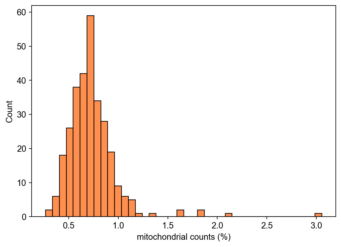
ax = sns.histplot(
    adata.obs,
    x="pct_counts_ribo",
    color="#ff6a14",
)
ax.set_xlabel("ribosomal counts (%)")
Text(0.5, 0, 'ribosomal counts (%)')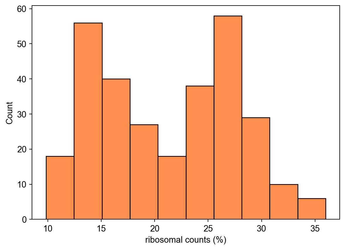
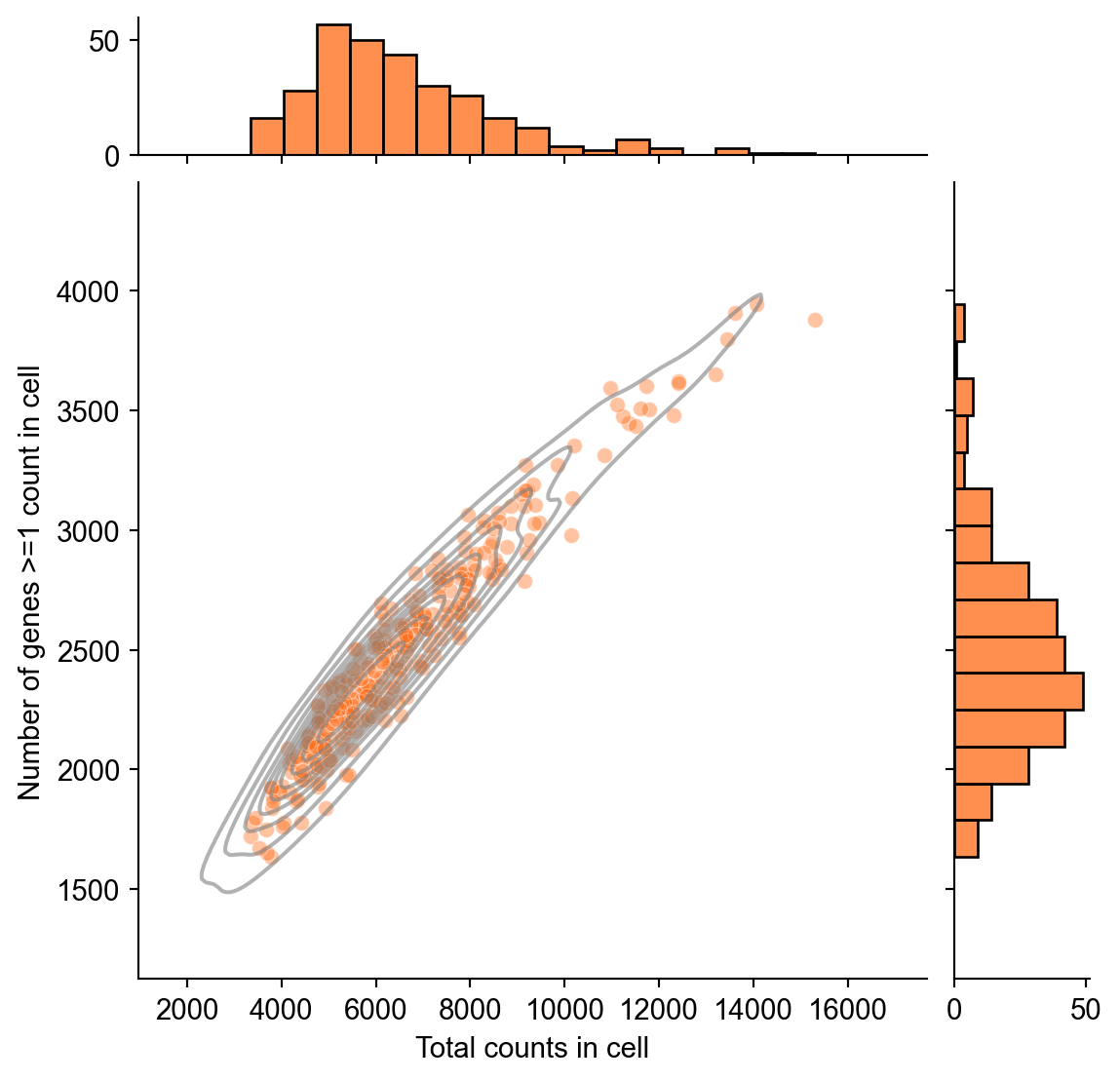
as well as the number of genes with at least one count in each cell and the total counts in each cell.
import seaborn as sns
import pandas as pd

numeric_obs = adata.obs.copy()
numeric_obs["n_genes_by_counts"] = pd.to_numeric(
    numeric_obs["n_genes_by_counts"],
    errors="coerce",
)
qc_counts = sns.jointplot(
    data=numeric_obs,
    x="total_counts",
    y="n_genes_by_counts",
    color="#ff6a14",
    marginal_ticks=True,
    kind="scatter",
    alpha=0.4,
)
qc_counts.plot_joint(
    sns.kdeplot,
    color="gray",
    alpha=0.6,
)
qc_counts.set_axis_labels(
    xlabel="Total counts in cell",
    ylabel="Number of genes >=1 count in cell",
)
For some data sets we apply cytotrace as a proxy for progression through lineage-specific differentiation.
from pyrovelocity.analysis.cytotrace import cytotrace_sparse

cytotrace_sparse(adata, layer="spliced")
cytotrace_representation = anndata_string(adata)
print_string_diff(
    text1=copied_raw_counts_representation,
    text2=cytotrace_representation,
    diff_title="Cytotrace diff",
)
╭────────────── Cytotrace diff ───────────────╮ │ │ │ --- +++ @@ -7,8 +7,25 @@ G2M_score, │ │ u_lib_size_raw, │ │ s_lib_size_raw, │ │ + n_genes_by_counts, │ │ + total_counts, │ │ + total_counts_mt, │ │ + pct_counts_mt, │ │ + total_counts_ribo, │ │ + pct_counts_ribo, │ │ + gcs, │ │ + cytotrace, │ │ + counts, │ │ var: │ │ highly_variable_genes, │ │ + mt, │ │ + ribo, │ │ + n_cells_by_counts, │ │ + mean_counts, │ │ + pct_dropout_by_counts, │ │ + total_counts, │ │ + cytotrace, │ │ + cytotrace_corrs, │ │ uns: │ │ clusters_coarse_colors, │ │ clusters_colors, │ │ │ │ │ ╰─────────────────────────────────────────────╯
Next we use the preprocessing functions built-in to the scvelo package to filter genes that have at least a given minimum number of counts,
import scvelo as scv

scv.pp.filter_genes(
    adata,
    min_shared_counts=30,
)
filter_genes_representation = anndata_string(adata)
print_string_diff(
    text1=cytotrace_representation,
    text2=filter_genes_representation,
    diff_title="Filter genes diff",
)
Filtered out 26305 genes that are detected 30 counts (shared).╭──────────────── Filter genes diff ────────────────╮ │ │ │ --- +++ @@ -1,5 +1,5 @@ │ │ -AnnData object with n_obs × n_vars = 300 × 27998 │ │ +AnnData object with n_obs × n_vars = 300 × 1693 │ │ obs: │ │ clusters_coarse, │ │ clusters, │ │ @@ -16,6 +16,9 @@ gcs, │ │ cytotrace, │ │ counts, │ │ + initial_size_unspliced, │ │ + initial_size_spliced, │ │ + initial_size, │ │ var: │ │ highly_variable_genes, │ │ mt, │ │ │ │ │ ╰───────────────────────────────────────────────────╯
normalize the data,
scv.pp.normalize_per_cell(adata)
normalize_representation = anndata_string(adata)
print_string_diff(
    text1=filter_genes_representation,
    text2=normalize_representation,
    diff_title="Normalize per cell diff",
)
Normalized count data: X, spliced, unspliced.╭───────────────── Normalize per cell diff ─────────────────╮ │ │ │ --- +++ @@ -19,6 +19,7 @@ initial_size_unspliced, │ │ initial_size_spliced, │ │ initial_size, │ │ + n_counts, │ │ var: │ │ highly_variable_genes, │ │ mt, │ │ │ │ │ ╰───────────────────────────────────────────────────────────╯
and filter the genes by their degree of dispersion.
scv.pp.filter_genes_dispersion(
    adata,
    n_top_genes=2000,
)
filter_dispersion_representation = anndata_string(adata)
print_string_diff(
    text1=normalize_representation,
    text2=filter_dispersion_representation,
    diff_title="Filter dispersion diff",
)
Skip filtering by dispersion since number of variables are less than `n_top_genes`.╭─ Filter dispersion diff ─╮ │ │ │ │ │ │ ╰──────────────────────────╯
Aside from the observation-level subsampling these operations are destructive and so you would need to reload the data to recover its original state after attempting to apply them.
Finally we use the scanpy package to log-transform the data. Note again we’ve retained the count data and are only doing this as it is expected by a variety of downstream analysis tools.
import scanpy as sc

sc.pp.log1p(adata)
preprocessed_data_state_representation = anndata_string(adata)
print_string_diff(
    text1=filter_dispersion_representation,
    text2=preprocessed_data_state_representation,
    diff_title="Log transform diff",
)
╭───────────── Log transform diff ──────────────╮ │ │ │ --- +++ @@ -36,6 +36,7 @@ day_colors, │ │ neighbors, │ │ pca, │ │ + log1p, │ │ obsm: │ │ X_pca, │ │ X_umap, │ │ │ │ │ ╰───────────────────────────────────────────────╯
Having executed this series of functions we’ve added or updated the following components relative to the initial data state
print_string_diff(
    text1=initial_data_state_representation,
    text2=preprocessed_data_state_representation,
    diff_title="Filtration and normalization summary diff",
    diff_context_lines=5,
)
╭──── Filtration and normalization summary diff ─────╮ │ │ │ --- +++ @@ -1,24 +1,50 @@ │ │ -AnnData object with n_obs × n_vars = 3696 × 27998 │ │ +AnnData object with n_obs × n_vars = 300 × 1693 │ │ obs: │ │ clusters_coarse, │ │ clusters, │ │ S_score, │ │ G2M_score, │ │ + u_lib_size_raw, │ │ + s_lib_size_raw, │ │ + n_genes_by_counts, │ │ + total_counts, │ │ + total_counts_mt, │ │ + pct_counts_mt, │ │ + total_counts_ribo, │ │ + pct_counts_ribo, │ │ + gcs, │ │ + cytotrace, │ │ + counts, │ │ + initial_size_unspliced, │ │ + initial_size_spliced, │ │ + initial_size, │ │ + n_counts, │ │ var: │ │ highly_variable_genes, │ │ + mt, │ │ + ribo, │ │ + n_cells_by_counts, │ │ + mean_counts, │ │ + pct_dropout_by_counts, │ │ + total_counts, │ │ + cytotrace, │ │ + cytotrace_corrs, │ │ uns: │ │ clusters_coarse_colors, │ │ clusters_colors, │ │ day_colors, │ │ neighbors, │ │ pca, │ │ + log1p, │ │ obsm: │ │ X_pca, │ │ X_umap, │ │ layers: │ │ spliced, │ │ unspliced, │ │ + raw_unspliced, │ │ + raw_spliced, │ │ obsp: │ │ distances, │ │ connectivities, │ │ │ ╰────────────────────────────────────────────────────╯
We do not make direct use of nearest neighbor graphs, and some data sets come with one precomputed, but we recompute the graph for cross-compatability with other tools that may require it.
sc.pp.neighbors(
    adata=adata,
    n_pcs=30,
    n_neighbors=30,
)
nearest_neighbors_representation = anndata_string(adata)
print_string_diff(
    text1=preprocessed_data_state_representation,
    text2=nearest_neighbors_representation,
    diff_title="Nearest neighbors diff",
)
╭─ Nearest neighbors diff ─╮ │ │ │ │ │ │ ╰──────────────────────────╯
The nearest neighbor graph is used in particular for nearest-neighbor-based averaging of gene expression
scv.pp.moments(
    data=adata,
    n_pcs=30,
    n_neighbors=30,
)
nearest_neighbor_averaged_representation = anndata_string(adata)
print_string_diff(
    text1=nearest_neighbors_representation,
    text2=nearest_neighbor_averaged_representation,
    diff_title="Nearest neighbor averaged diff",
)
computing moments based on connectivities
finished (0:00:00) --> added
'Ms' and 'Mu', moments of un/spliced abundances (adata.layers)╭─────── Nearest neighbor averaged diff ───────╮ │ │ │ --- +++ @@ -45,6 +45,8 @@ unspliced, │ │ raw_unspliced, │ │ raw_spliced, │ │ + Ms, │ │ + Mu, │ │ obsp: │ │ distances, │ │ connectivities, │ │ │ ╰──────────────────────────────────────────────╯
We compute the estimates of the expression dynamics parameters using the EM-based maximum-likelihood algorithm from the scvelo package
scv.tl.recover_dynamics(
    data=adata,
    n_jobs=-1,
    use_raw=False,
)
em_ml_dynamics_representation = anndata_string(adata)
print_string_diff(
    text1=nearest_neighbor_averaged_representation,
    text2=em_ml_dynamics_representation,
    diff_title="EM ML dynamics diff",
)
recovering dynamics (using 16/16 cores)
finished (0:00:03) --> added
'fit_pars', fitted parameters for splicing dynamics (adata.var)╭────────────── EM ML dynamics diff ───────────────╮ │ │ │ --- +++ @@ -30,6 +30,22 @@ total_counts, │ │ cytotrace, │ │ cytotrace_corrs, │ │ + fit_r2, │ │ + fit_alpha, │ │ + fit_beta, │ │ + fit_gamma, │ │ + fit_t_, │ │ + fit_scaling, │ │ + fit_std_u, │ │ + fit_std_s, │ │ + fit_likelihood, │ │ + fit_u0, │ │ + fit_s0, │ │ + fit_pval_steady, │ │ + fit_steady_u, │ │ + fit_steady_s, │ │ + fit_variance, │ │ + fit_alignment_scaling, │ │ uns: │ │ clusters_coarse_colors, │ │ clusters_colors, │ │ @@ -37,9 +53,12 @@ neighbors, │ │ pca, │ │ log1p, │ │ + recover_dynamics, │ │ obsm: │ │ X_pca, │ │ X_umap, │ │ + varm: │ │ + loss, │ │ layers: │ │ spliced, │ │ unspliced, │ │ @@ -47,6 +66,9 @@ raw_spliced, │ │ Ms, │ │ Mu, │ │ + fit_t, │ │ + fit_tau, │ │ + fit_tau_, │ │ obsp: │ │ distances, │ │ connectivities, │ │ │ ╰──────────────────────────────────────────────────╯
and use these to estimate the gene-specific velocities.
scv.tl.velocity(
    data=adata,
    mode="dynamical",
    use_raw=False,
)
em_ml_velocities_representation = anndata_string(adata)
print_string_diff(
    text1=em_ml_dynamics_representation,
    text2=em_ml_velocities_representation,
    diff_title="EM ML velocities diff",
)
computing velocities
finished (0:00:00) --> added
'velocity', velocity vectors for each individual cell (adata.layers)╭───────────── EM ML velocities diff ─────────────╮ │ │ │ --- +++ @@ -46,6 +46,7 @@ fit_steady_s, │ │ fit_variance, │ │ fit_alignment_scaling, │ │ + velocity_genes, │ │ uns: │ │ clusters_coarse_colors, │ │ clusters_colors, │ │ @@ -54,6 +55,7 @@ pca, │ │ log1p, │ │ recover_dynamics, │ │ + velocity_params, │ │ obsm: │ │ X_pca, │ │ X_umap, │ │ @@ -69,6 +71,8 @@ fit_t, │ │ fit_tau, │ │ fit_tau_, │ │ + velocity, │ │ + velocity_u, │ │ obsp: │ │ distances, │ │ connectivities, │ │ │ ╰─────────────────────────────────────────────────╯
We add leiden clustering to the data set for algorithms that work with unlabeled clusters.
sc.tl.leiden(adata=adata)
leiden_representation = anndata_string(adata)
print_string_diff(
    text1=em_ml_velocities_representation,
    text2=leiden_representation,
    diff_title="Leiden clustering diff",
)
╭──────────────── Leiden clustering diff ─────────────────╮ │ │ │ --- +++ @@ -20,6 +20,7 @@ initial_size_spliced, │ │ initial_size, │ │ n_counts, │ │ + leiden, │ │ var: │ │ highly_variable_genes, │ │ mt, │ │ @@ -56,6 +57,7 @@ log1p, │ │ recover_dynamics, │ │ velocity_params, │ │ + leiden, │ │ obsm: │ │ X_pca, │ │ X_umap, │ │ │ │ │ ╰─────────────────────────────────────────────────────────╯
We also subset the genes to a smaller number to enable faster illustration of model training and inference even on laptops with significantly limited resources.
likelihood_sorted_genes = (
    adata.var["fit_likelihood"].sort_values(ascending=False).index
)

if PYROVELOCITY_DATA_SUBSET:
    adata = adata[:, likelihood_sorted_genes[:200]].copy()

subset_genes_representation = anndata_string(adata)
print_string_diff(
    text1=leiden_representation,
    text2=subset_genes_representation,
    diff_title="Subset genes diff",
)
╭─────────────── Subset genes diff ────────────────╮ │ │ │ --- +++ @@ -1,5 +1,5 @@ │ │ -AnnData object with n_obs × n_vars = 300 × 1693 │ │ +AnnData object with n_obs × n_vars = 300 × 200 │ │ obs: │ │ clusters_coarse, │ │ clusters, │ │ │ │ │ ╰──────────────────────────────────────────────────╯
We compute the velocity graph based on cosine similarity of the gene-specific velocities estimated by the scvelo package.
scv.tl.velocity_graph(
    data=adata,
    n_jobs=-1,
)
velocity_graph_representation = anndata_string(adata)
print_string_diff(
    text1=subset_genes_representation,
    text2=velocity_graph_representation,
    diff_title="Velocity graph diff",
)
computing velocity graph (using 16/16 cores)
finished (0:00:00) --> added
'velocity_graph', sparse matrix with cosine correlations (adata.uns)╭────────────── Velocity graph diff ──────────────╮ │ │ │ --- +++ @@ -21,6 +21,7 @@ initial_size, │ │ n_counts, │ │ leiden, │ │ + velocity_self_transition, │ │ var: │ │ highly_variable_genes, │ │ mt, │ │ @@ -58,6 +59,8 @@ recover_dynamics, │ │ velocity_params, │ │ leiden, │ │ + velocity_graph, │ │ + velocity_graph_neg, │ │ obsm: │ │ X_pca, │ │ X_umap, │ │ │ │ │ ╰─────────────────────────────────────────────────╯
We compute the velocity embedding using the velocity graph and the gene-specific velocities.
scv.tl.velocity_embedding(
    data=adata,
    basis="umap",
)
velocity_embedding_representation = anndata_string(adata)
print_string_diff(
    text1=velocity_graph_representation,
    text2=velocity_embedding_representation,
    diff_title="Velocity embedding diff",
)
computing velocity embedding
finished (0:00:00) --> added
'velocity_umap', embedded velocity vectors (adata.obsm)╭────── Velocity embedding diff ──────╮ │ │ │ --- +++ @@ -64,6 +64,7 @@ obsm: │ │ X_pca, │ │ X_umap, │ │ + velocity_umap, │ │ varm: │ │ loss, │ │ layers: │ │ │ │ │ ╰─────────────────────────────────────╯
We compute the gene-specific latent time estimated by the scvelo package.
scv.tl.latent_time(
    data=adata,
)
latent_time_representation = anndata_string(adata)
print_string_diff(
    text1=velocity_embedding_representation,
    text2=latent_time_representation,
    diff_title="Latent time diff",
)
computing terminal states
identified 2 regions of root cells and 1 region of end points .
finished (0:00:00) --> added
'root_cells', root cells of Markov diffusion process (adata.obs)
'end_points', end points of Markov diffusion process (adata.obs)
computing latent time using root_cells as prior
finished (0:00:00) --> added
'latent_time', shared time (adata.obs)╭────────────── Latent time diff ──────────────╮ │ │ │ --- +++ @@ -22,6 +22,10 @@ n_counts, │ │ leiden, │ │ velocity_self_transition, │ │ + root_cells, │ │ + end_points, │ │ + velocity_pseudotime, │ │ + latent_time, │ │ var: │ │ highly_variable_genes, │ │ mt, │ │ │ │ │ ╰──────────────────────────────────────────────╯
We can finally summarize the changes induced by the preprocessing steps applied to the data set.
print_string_diff(
    text1=initial_data_state_representation,
    text2=latent_time_representation,
    diff_title="Preprocessing summary diff",
    diff_context_lines=5,
)
╭──────────── Preprocessing summary diff ────────────╮ │ │ │ --- +++ @@ -1,24 +1,88 @@ │ │ -AnnData object with n_obs × n_vars = 3696 × 27998 │ │ +AnnData object with n_obs × n_vars = 300 × 200 │ │ obs: │ │ clusters_coarse, │ │ clusters, │ │ S_score, │ │ G2M_score, │ │ + u_lib_size_raw, │ │ + s_lib_size_raw, │ │ + n_genes_by_counts, │ │ + total_counts, │ │ + total_counts_mt, │ │ + pct_counts_mt, │ │ + total_counts_ribo, │ │ + pct_counts_ribo, │ │ + gcs, │ │ + cytotrace, │ │ + counts, │ │ + initial_size_unspliced, │ │ + initial_size_spliced, │ │ + initial_size, │ │ + n_counts, │ │ + leiden, │ │ + velocity_self_transition, │ │ + root_cells, │ │ + end_points, │ │ + velocity_pseudotime, │ │ + latent_time, │ │ var: │ │ highly_variable_genes, │ │ + mt, │ │ + ribo, │ │ + n_cells_by_counts, │ │ + mean_counts, │ │ + pct_dropout_by_counts, │ │ + total_counts, │ │ + cytotrace, │ │ + cytotrace_corrs, │ │ + fit_r2, │ │ + fit_alpha, │ │ + fit_beta, │ │ + fit_gamma, │ │ + fit_t_, │ │ + fit_scaling, │ │ + fit_std_u, │ │ + fit_std_s, │ │ + fit_likelihood, │ │ + fit_u0, │ │ + fit_s0, │ │ + fit_pval_steady, │ │ + fit_steady_u, │ │ + fit_steady_s, │ │ + fit_variance, │ │ + fit_alignment_scaling, │ │ + velocity_genes, │ │ uns: │ │ clusters_coarse_colors, │ │ clusters_colors, │ │ day_colors, │ │ neighbors, │ │ pca, │ │ + log1p, │ │ + recover_dynamics, │ │ + velocity_params, │ │ + leiden, │ │ + velocity_graph, │ │ + velocity_graph_neg, │ │ obsm: │ │ X_pca, │ │ X_umap, │ │ + velocity_umap, │ │ + varm: │ │ + loss, │ │ layers: │ │ spliced, │ │ unspliced, │ │ + raw_unspliced, │ │ + raw_spliced, │ │ + Ms, │ │ + Mu, │ │ + fit_t, │ │ + fit_tau, │ │ + fit_tau_, │ │ + velocity, │ │ + velocity_u, │ │ obsp: │ │ distances, │ │ connectivities, │ │ │ ╰────────────────────────────────────────────────────╯
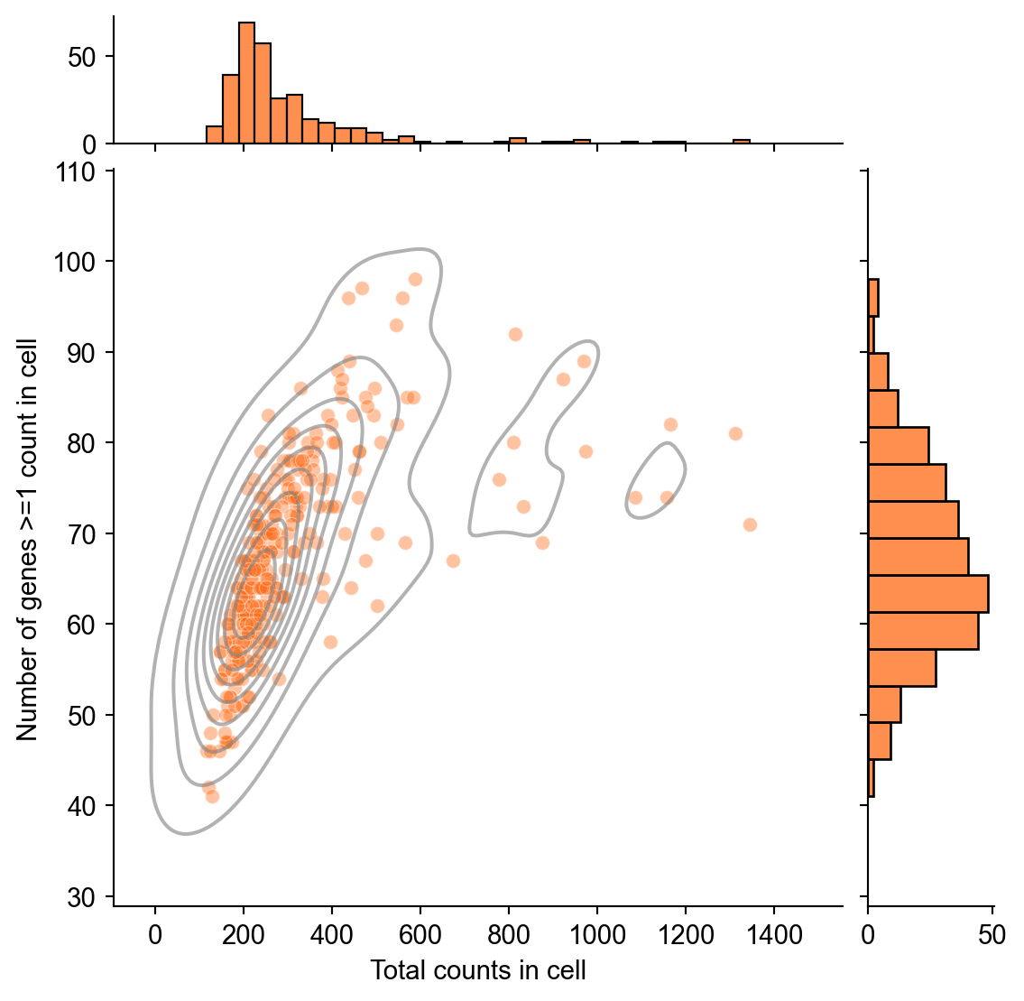
We plot the two-dimensional density of genes with greater than or equal to one count in a given cell versus the total counts in that cell for the data set.
sc.pp.calculate_qc_metrics(
    adata=adata,
    qc_vars=["mt", "ribo"],
    layer="raw_spliced",
    percent_top=None,
    log1p=False,
    inplace=True,
)
qc_metrics_representation = anndata_string(adata)
print_string_diff(
    text1=latent_time_representation,
    text2=qc_metrics_representation,
    diff_title="Quality control metrics diff",
)
╭─ Quality control metrics diff ─╮ │ │ │ │ │ │ ╰────────────────────────────────╯
import seaborn as sns
import pandas as pd

numeric_obs = adata.obs.copy()
numeric_obs["n_genes_by_counts"] = pd.to_numeric(
    numeric_obs["n_genes_by_counts"],
    errors="coerce",
)
qc_counts = sns.jointplot(
    data=numeric_obs,
    x="total_counts",
    y="n_genes_by_counts",
    color="#ff6a14",
    marginal_ticks=True,
    kind="scatter",
    alpha=0.4,
)
qc_counts.plot_joint(
    sns.kdeplot,
    color="gray",
    alpha=0.6,
)
qc_counts.set_axis_labels(
    xlabel="Total counts in cell",
    ylabel="Number of genes >=1 count in cell",
)
We can plot the raw data to ensure we have a general understanding of its sparsity, which may be associated with quality. We can also plot the raw spliced and unspliced counts.
from pyrovelocity.plots import plot_spliced_unspliced_histogram

chart = plot_spliced_unspliced_histogram(
    adata=adata,
    spliced_layer="raw_spliced",
    unspliced_layer="raw_unspliced",
    min_count=3,
    max_count=200,
)
chart.save("us_histogram.pdf")
chart